Chapter 2: Preferences

So far we have only considered what a consumer can afford. We aren’t saying anything yet about what the consumer actually wants. In order to do this we’ll need to introduce consumer preferences

Suppose we have two bundles, (x1, x2) and (y1, y2). We say the consumer strictly prefers bundle X to Y and write:

\((x_1, x_2) \succ (y_1, y_2)\)

We say the consumer weakly prefers bundle X to Y and write:

\((x_1, x_2) \succeq (y_1, y_2)\)

We say the consumer is indifferent between bundles X & Y and write:

\((x_1, x_2) \sim (y_1, y_2)\)

We say preferences are complete when any two bundles can be compared. For any two bundles either (x1, x2) ≽ (y1, y2) or (y1, y2) ≽ (x1, x2) or both i.e. (x1, x2) ∼ (y1, y2)

We say preferences are reflexive when any bundle is at least as good as itself. For any bundle (x1, x2) ≽ (x1, x2)

We say preferences are transitive when if bundle A is preferred to B, and B is preferred to C, then A is preferred to C. For any three bundles X,Y,&Z: (x1,x2) ≽ (y1,y2) and (y1, y2) ≽ (z1, z2) implies (x1, x2) ≽ (z1, z2)

Suppose we pick an arbitrary bundle, (x1,x2). We say all of the bundles weakly preferred to (x1,x2) is the consumer’s weakly preferred set. We say the bundles the consumer likes as much as (x1,x2) make up an indifference curve. Indifference curves form the boundary to the weakly preferred set

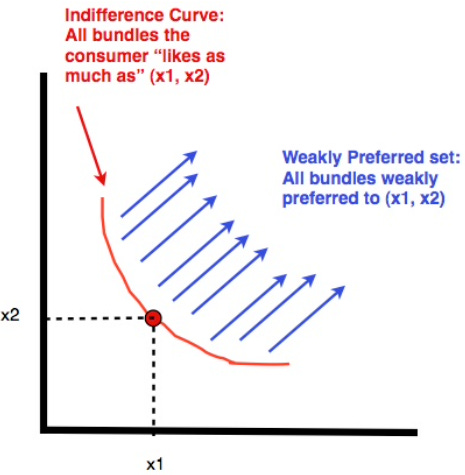
An indifference curve through a bundle consists of all other bundles that leave the consumer indifferent to that given bundle. Sometimes it’s helpful to draw arrows in the direction of the preferred bundles. We allow many shapes of indifference curves but we definitely require that indifference curves never cross. Why?

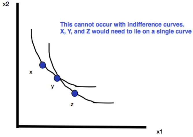
The issue we run into with crossing indifference curve like those shown above is a violation of transitivity. Since bundle X and bundle Y lie on the same indifference curve they must be liked as well as each other. But Y and Z are also on the same indifference curve so the consumer must like Y and Z the same. However, there’s a portion from the indifference curve that X lies on that crosses into the weekly preferred set of the indifference curve that Z lies on. So those bundles must be preferred to Z which is a contradiction because they’re as good as Y which is supposed to be as good as Z!

Examples of indifference curves that represent known economic concepts:

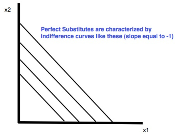
Two goods are perfect substitutes if the consumer will substitute one good for the other at a constant rate. An example is one for one substitution. The key characteristic is indifference curves with a constant slope, i.e. straight line

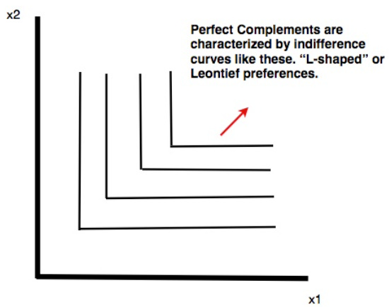
Two goods are perfect complements if they are always consumed together in fixed proportions. Indifference curves are L-shaped where the vertex occurs where the number of good one equals the number of good 2. Increasing both quantities at the same time moves the consumer to a higher indifference curve. The fixed proportion need not be 1-1.

Substitutes and complements preferences arise pretty frequently in intermediate microeconomics level analysis. But it’s also helpful to represent some less encountered preference shapes to better reinforce our understanding of preferences and indifference curves.

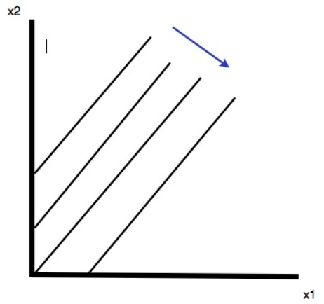
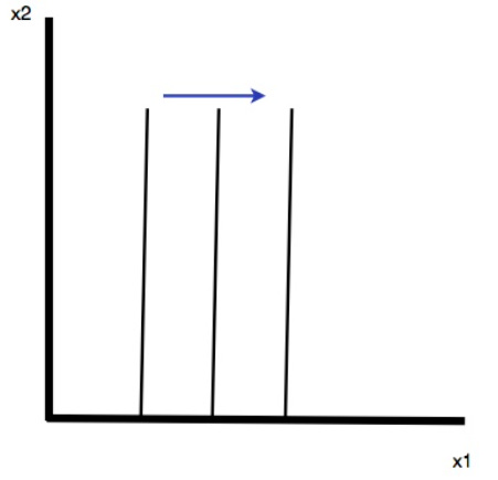
A commodity is a bad if the consumer does not like it. Indifference curves have a positive slope. The interpretation of the positive slope follows from the idea that in order to tolerate good 2 the consumer needs to be given more of good 1. A good is a neutral good if the consumer doesn’t care one way or the other. If x1 is a normal good, and x2 is neutral good then indifference curves are vertical

Exercise: If there are only two goods and if more of x1 is always preferred to less while less of x2 is always preferred to more, then what will the indifference curves for this consumer look like?

Answer:

We can also draw indifference curves for neutral goods:

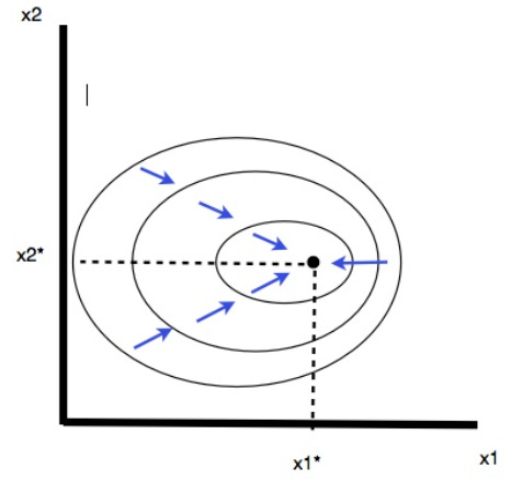
Satiation occurs where there is an overall best bundle for the consumer and the ‘closer’ they are to that best bundle the better off they are in terms of their own preferences. Suppose (x1,x2) is a most preferred bundle. The further from this bundle, the worse off the consumer is. Then (x1,x2) is called a satiation point or bliss point

Indifference curves have both a positive and negative slope:

1. Negative slope when consumer has too little or too much of both goods (too much of both means both are bads)

2.  Positive slope when too much of one goods (it becomes a bad, reducing consumption is better)

We definitely have to rule out satiation points for our analysis. In fact apart from substitutes and complements preferences, we’ll generally make some assumptions about the type of features we’ll want to consider and call the result well-behaved preferences.

1. Typically we assume that ‘more is better’

   1. This is called ‘monotonicity’ of preferences

   2.  If (x1,x2) is a bundle and (y1,y2) is a bundle of goods with at

   least as much of both goods and more of one, then

   (y1, y2) ≻ (x1, x2)

   c. We assume we’re considering points before satiation occurs

   d. This assumption implies that indifference curves will have a

   negative slope

Convex preferences: Averages are preferred to extremes:

We also assume that averages are preferred to extremes

1.  If two bundles on the same indifference curve (x1,x2) and (y1,y2), their weighted average (12x1 + 12y1, 12x2 + 12y2), is at least as good or strictly preferred.

   1.  This means that the set of bundles weakly preferred to (x1,x2) is a convex set.

   2. A convex set has the property that if you take any two point in the set and draw the line segment connecting the two, the segment lies entirely within the set

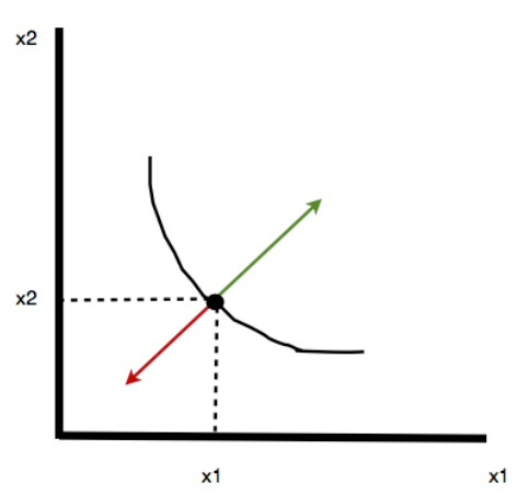
Marginal rate of substitution:

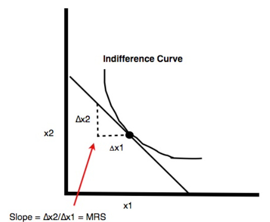
The marginal rate of substitution is the slope of an indifference curve at a particular point. It is a measure of the rate at which the consumer is just willing to substitute one good for the other. What we’re doing is taking a little of good one away, ∆x1, and replacing it with a little of good two, ∆x2, to keep them indifferent. As these amounts become infinitesimal the ratio ∆x2/∆x1 approaches the slope of indifference curve

Clearly we’re going to want to use calculus!

Since indifference curves typically have negative slopes, the sign of the MRS is often negative

Diminishing Marginal Rate of Substitution

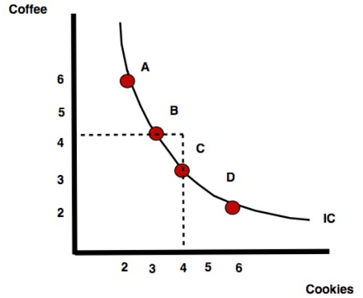
Referring to the picture on the last slide observe that the MRS varies along the curve. Just intuitively:

1. Point A: I have a lot of coffee and will gladly trade some for cookies

2. Point D: I have very little coffee and am reluctant to give any up for

   additional cookies.
   Let’s look more closely at the following potential trades and observe that MRS

   decreases as x1 (cookies) increases:

   1.  A to B:[(2,6)to(3,4)]: Giving up 2 coffee and I can be as happy replacing it with 1 cookie therefore MRS = 2

   2. B to C:[(3,4)to(4,3)]: Giving up 1 coffee and I can be as happy replacing it with 1 cookie therefore MRS = 1

   3.  C to D: [(4, 3) to (6,2)]: up 1 coffee and I can be as happy replacing it with 2 cookies therefore MRS = 1/2

See also: