Chapter 11: Monopoly

In economics classes when we refer to monopoly profit maximization we usually have a single price in mind. Generally we refer to the monopoly price to mean that which corresponds to the quantity where marginal revenue equals marginal cost. Later we’ll consider more sophisticated pricing schemes where a firm with market power offers multiple prices as in the case of price discrimination and even multiple types of prices as in the case of two-part tariff (two-part pricing). For now we’ll start with just the basic monopoly profit maximization problem:

The monopoly seeks to maximize profit by selecting the optimal quantity. As a cue to the structure of the problem we know we’re going to take a derivative to address the goal of maximization (optimization) and this derivative is with respect to quantity since that’s the variable that the monopoly is controlling, at least when the problem is structured this way. To make this happen we need to write out profits only as a function of quantity:

Profit(Q) = TR(Q) - TC(Q)

Profit(Q) = P(Q)*Q - C(Q)

In the above line I have replaced total revenue with its two components written as a product, price times quantity. The P(Q) indicates that price is a function of quantity and specifically this should remind you of inverse demand. This is necessary to generate profit only in terms of quantity.

From this point we can differentiate with respect to quantity, set equal to zero to generate our first order condition, and then solve to find the profit maximizing quantity (for a single-price monopoly).

dProfit/dQ = dP/dQ*Q + P*dQ/dQ - dC/dQ = 0

dProfit/dQ = dP/dQ*Q +P =MC

This isn’t so useful to see in abstract form so I’ll introduce a numerical example shortly. But first I want to point out that we can turn this jumble of letters into a useful equation. We have:

(dP/dQ)*Q + P = MC

And can write:

-(dP/dq)*Q = P-MC

I wrote it this way because P-MC has a useful interpretation: it’s just ‘mark-up’ which captures how much higher price is than marginal cost. P-MC is just some numerical value but alone isn’t so useful in absolute terms. Clearly P-MC = 1 is a more significant mark up if P=2 and MC=1 than if P=101 and MC=100. So let’s divide through by price to generate a ‘percentage mark-up’.

-(dP/dQ)(Q/P) = (P-MC)/P

Written this way you might not immediately recognize it, but the left hand term is just the reciprocal of price elasticity of demand. Price elasticity is just the percentage change in quantity divided by the percentage change in price. That’s just: dQ/Q / dP/P then written as: dQ/Q * P/dP or dQ/dP * P/Q which is the reciprocal of what we had above! So finally we can write:

-1/E = (P-MC)/P where E is price elasticity of demand. This tells us we can relate the percentage mark-up with the price elasticity of demand. The more elastic is demand, the lower the mark-up. In the extreme if demand is perfectly elastic mark-up is zero, exactly as predicted in a perfectly competitive market. Note this formula only works for elastic demand and not for inelastic demand. That’s because MR is negative on the inelastic portion of demand.

Here’s a numerical example for monopoly profit maximization:

Let P = 10 - Q and MC=2. Then we write:

Profit = (10-Q)Q - 2Q

Profit = 10Q - Q^2 - 2Q

dProfit/dQ = 10 - 2q - 2 = 0

8 - 2q

q=4

Then P=10-(4) = 6.

So the profit maximizing quantity is q*=4 and price is p*=6.

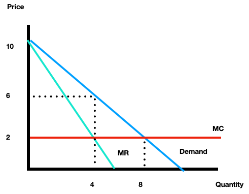
While the profit maximizing point occurs where the firm produces 4 units and sells each at the single price of $6, the revenue maximizing point is a quantity of 5 units at a price of $5. Actually because of an important fact no calculations are necessary to find the revenue maximizing point: Revenue is maximized at the midpoint of the demand curve. If we were to maximize revenue we would take dTR/dq and set equal to zero to find the first order condition. That’s just MR=0. However, inspecting the above graph we see that MR=0 at the point (5,0) which corresponds to a quantity of 5. When marginal costs are zero the revenue maximizing outcome is the profit maximizing solution, because Profit is TR - TC and maximized where MR-MC = 0 but if MC=0 we have only: MR=0. Also recall (hopefully) from introductory microeconomics that demand is unit elastic at the midpoint of the demand curve.

From this point there’s two other useful details: We can compare the monopoly profit maximizing outcome to the competitive market outcome. We can complete the welfare analysis by computing consumer and producer surplus. The competitive outcome assumes there’s many sellers in the market each producing the quantity that brings its marginal cost equal to 2. Why is this? Remember, the competitive market assumes that firms are price takers. They cannot influence the price, but can only respond to it. When faced with a particular market price the competitive firm determines how much to optimally produce by watching how its marginal cost changes as it increases or decreases production. Since all units are therefore sold for a constant price equal to the market price, the marginal revenue for each unit is just the market price. All firms that sell at a single price will find the optimal level of output at the point where marginal revenue equals marginal cost. So the firm adjusts is output until marginal cost equals marginal revenue.

To make comparison to the monopoly firm serving the entire market as a whole we need to solve this problem at the industry level by setting the market demand curve equal to the marginal cost. In this example this is just: P=10 - Q = 2 = MC and solving we find Q = 8 with of course P=2. Notice that the competitive firm produces considerably more than a monopoly firm, in this case exactly double the output. The fact that the competitive output is double the monopoly output is not a general truth, but an artifact of this particular type of demand curve and marginal cost curve. We also see that the monopoly sets a higher price. The difference between price and marginal cost is ‘mark-up’ which in this case is $4 for the monopoly and $0 for any firm in a perfectly competitive market.

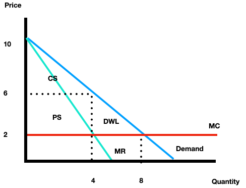
Seeing now that the monopoly produces less and charges more than a competitive firm, we can better determine the cost of the monopoly in the sense of inefficiency by comparing consumer and producer surplus in the monopoly and competitive market cases. Remember the definitions of consumer and producer surplus:

Consumer surplus is the economic value generated through market activity and received by consumers. It’s the difference between the willingness to pay of consumers and the price they actually pay. Graphically it’s the area below the demand curve and above the marginal cost curve.

Producer surplus is the economic value generated through market activity and received by producers. It’s the difference between the price the good or service is sold at and the marginal costs of producers. Graphically it’s the area beneath the market price and above the marginal cost. If there are no fixed costs, producer surplus and profits are the same thing (producer surplus only captures the variable portions).

We can compute each for the above example making use of simple area formulas. The area of a triangle is computed as 1/2 * Base * Height and in this example that’s the only one we require for consumer surplus.

CS = (1/2)(10 - 6)*(4-0)

CS = (1/2) (4)^2

CS = 8

The area of a square is computed as length * width and in this example it’s all we require to compute producer surplus: (6-2)(4-0), so PS = 16.

In the monopoly case there is inefficiency labeled on the graph as DWL for deadweight loss. It’s calculated in this case as the area of a triangle.

DWL = (1/2)(6-2)(8-4) = 8. Again, as just an artifact of these particular equations, consumer surplus and deadweight loss are equal but that is not true generally.

In the competitive market case there is no producer surplus. That’s because P=MC so we immediately see that (P-MC)(8-0) is just (2-2)(8) which is 0. There’s also no deadweight loss as the entire area under the demand curve and above the marginal cost is consumer surplus: CS= (1/2)(10 - 2)(8-0) = 32.

Note that the sum of the areas in the monopoly case, CS+PS+DWL = CS in the competitive case. This is a fairly large amount of inefficiency introduced by this monopoly, roughly 1/4 of the potential economic surplus in this market is lost as DWL (8/32 = 1/4). But this is a little misleading and warrants further reflection. Remember deadweight loss measures inefficiency specifically in the one particular market that we’re considering. There are other important considerations: People like variety but product differentiation brings us to different markets and introduces inefficiency. Sometimes a product or service cannot be profitably produced by a competitive market: It’s either monopoly or nothing!